Temperature sensors¶

One of the most important parameters for protecting a motor against overheating is the motor’s temperature. The motor temperature should be monitored to prevent over-temperature and damage to the motor winding.

Types of temperature sensors¶

Several types of sensors are well known and widely used in the industry:

Thermocouple
Thermistors
Resistance temperature detectors (RTDs)

Thermocouple¶

A thermocouple is an electrical device consisting of two dissimilar electrical conductors forming an electrical junction. A thermocouple produces a temperature-dependent voltage as a result of the thermoelectric effect.

Note

The generated voltage by a thermocouple is not enough to be measured by analog inputs and require an interface circuit (transducers) to increase the output voltage level.

Thermistors¶

PTC and NTC thermistors can be used as well, but NTC thermistors have the disadvantage that a wire brake can be confused with low temperatures.

Resistance temperature detectors¶

Resistance temperature detectors (RTDs) are manufactured from metals whose resistance increases with temperature.

SOMANET servo drives can directly measure the voltage or resistance so RTDs like KTY84-130 and PT1000 can be directly attached.

A wide range of RTD sensors can be measured by the temperature sensor input (SOMANET Circulo only) or analog inputs.

Note

This application note is focused on RTDs.

Pull-up resistor selection¶

For measuring the temperature using an RTD, the sensor’s voltage needs to be adjusted to a specific temperature range by adding a pull-up resistor.

The analog input can be configured to read the input voltage or input resistance. Subitem 0x2038:3 defines the value of the pull-up resistor. Two modes for measuring the analog input value can be distinguished:

Pull-up resistor (0x2038:3) = 0

The measured value will be the exact value of the analog input voltage.

0 = 0 volts and 4096 = full scale (according to the full scale voltage of the analog input)

Pull-up resistor (0x2038:3) > 0

In this mode, the firmware will calculate the resistor value (in Ω) connected to the input terminals. This feature is useful when using RTD sensors or another resistive sensor.

Note

RTDs with a minimum of 3 Ω resistance change per °C result in an acceptable accuracy.

According to the curves below, PT1000 and KTY-130 are good fitting sensors, both sensors are almost linear in the desired range.

../../../_images/curve_temp_pt1000_pt100.jpg

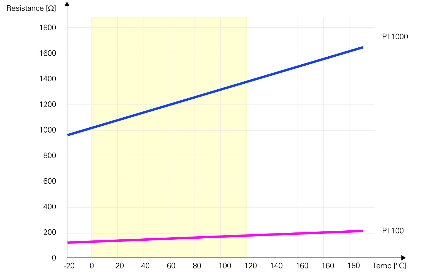
$\Rightarrow$ PT1000: 3.9 Ω per °C

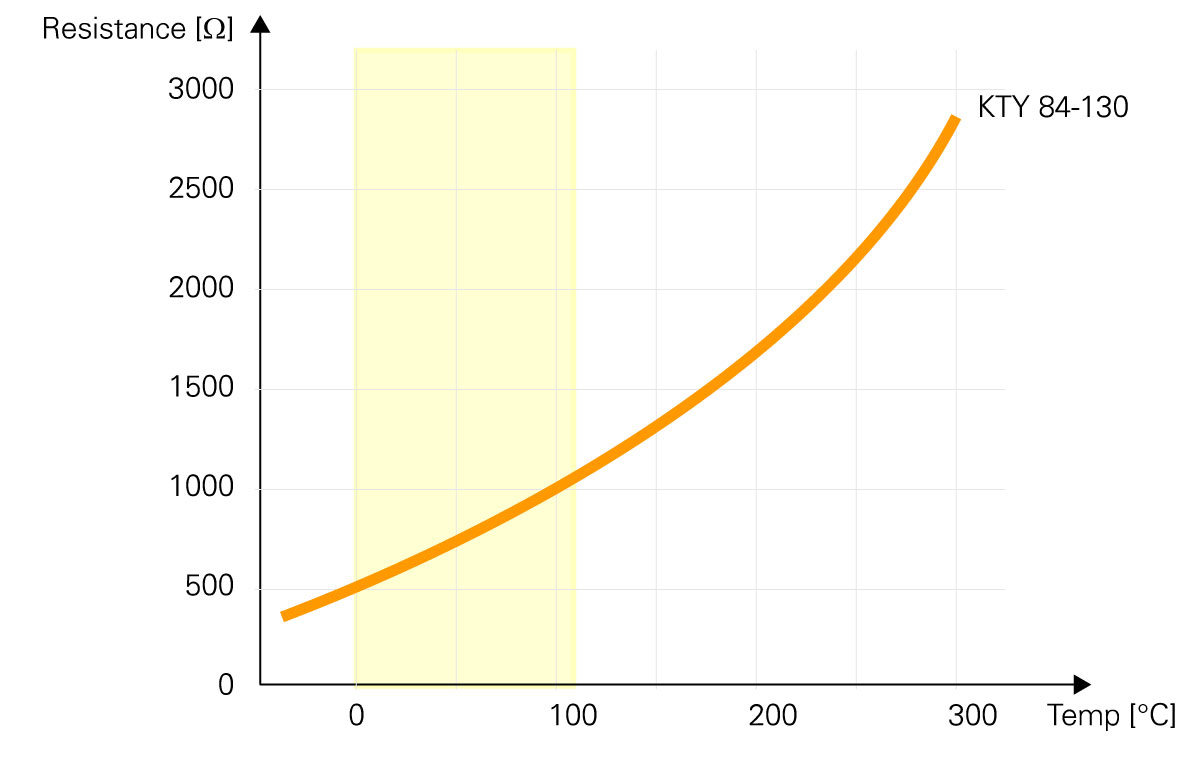
$\Rightarrow$ KYT 84-130: 5 Ω per °C

Note

Some analog inputs have a low input resistance. The internal input resistance is connected in parallel to the input.

Example: Measuring a motor temperature using a PT1000 temperature sensor

According to the PT1000 resistance table (provided, for example, from your sensor’s datasheet) the resistance of the sensor should be 1000 Ω for 0° C and 1385 Ω for 100° C.

The reference voltage is 5 V, and the ADC resolution is 12 bits, so the ADC output value would be 4095 for full scale input voltage.

The image below depicts a schematic of input circuits. The ADC will measure the input voltage which is proportional to the resistance.

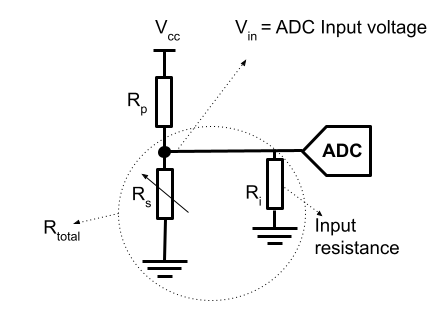
The sensor resistance and the input resistance are in parallel which means: R _total = $\frac {R_i \cdot R_s} {R_i + R_s}$

If the temperature sensor is used on the single-ended analog input of Circulo then R _s = R _total because R _i >> R _s.

The input voltage is = 5 V · $\frac {R_{total}} {R_p + R_{total}}$

To evaluate the accuracy, the amount of ticks for the measured temperature range needs to be considered: Temperature range / Amount of ticks for the temperature range = Temperature measured / tick

Example: ADC output on Circulo for a PT1000 temperature sensor

R _p = 4.7 kΩ, R _i be neglected because R _i >> R _s

ADC input voltage for 0° = 5 V · $\frac {1000~ \Omega} {4700~ \Omega + 1000~ \Omega}$ = 0.8772 V

ADC input voltage for 100° = 5 V · $\frac {1385~ \Omega} {4700~ \Omega + 1385~ \Omega}$ = 1.138 V

The converted value (ADC ticks) for 0° is = 4095 · $\frac {0.8772~ V} {5 V}$ = 718

The converted value (ADC ticks) for 100° is = 4095 · $\frac {1.138~ V} {5 V}$ = 932

Temperature range in ticks: 932 - 718 = 214 ticks for 100° C.

This leads to an accuracy of $\frac {100^{\circ}~ C} {214}$ ≈ 0.5° for measuring the temperature.

Now the accuracy of a PT100 with an R _p of 4.7 kΩ can be calculated for comparison:

Example: ADC output on Circulo for a PT100 temperature sensor.

ADC input voltage for 0° = 55 V · $\frac {100~ \Omega} {4700~ \Omega + 100~ \Omega}$ = 0.1042 V

ADC input voltage for 100° = 5 V · $\frac {139.16~ \Omega} {4700~ \Omega + 485~ \Omega}$ = 0.134 V

The converted value (ADC ticks) for 0° is = 4095 · $\frac {0.1042~ V} {5 V}$ = 85

The converted value (ADC ticks) for 100° is = 4095 · $\frac {0.468~ V} {5 V}$ = 110

Temperature range in ticks: 110 - 85 = 25 for 100°C

Accuracy: $\frac {100^{\circ}~ C} {25}$ = 4° for measuring the temperature.

Polynomial or Quintic function¶

After converting the analog input to digital, a five order polynomial function can be used to compensate the non-linearity of the input.

There are two methods for compensating the errors:

Using the master controller and perform the calculation on the master side.
Using the integrated polynomial function

$F(x) = a_5 \cdot x^5 + a_4 \cdot x^4 + a_3 \cdot x^3 + a_2 \cdot x^2 + a_1 \cdot x + a_0$

Note

The polynomial can only be used for one of the analog inputs.

Two methods are available:

Input voltage measurement
Input resistance measurement

Case 1: Input voltage measurement

The polynomial function can be used to compensate the non-linearity of the input voltage:

$y(V_{in}) = a_5 \cdot V_{in}^5 + a_4 \cdot V_{in}^4 + a_3 \cdot V_{in}^3 + a_2 \cdot V_{in}^2 + a_1 \cdot V_{in} + a_0$

Case 2: Input resistance measurement

When an RTD is used, the temperature is a function of the measured resistance:

$y(R) = a_5 \cdot R^5 + a_4 \cdot R^4 + a_3 \cdot R^3 + a_2 \cdot R^2 + a_1 \cdot R + a_0$

If the internal analog input is chosen with a pull-up resistor, the result of the calculation would be the resistor’s amount in Ω connected to the input terminals. With the coefficients set as a ₀ = 0, a ₁ = 1, a ₂ = 0, a ₃ = 0, a ₄ = 0, a ₅ = 0 the result equals the exact value of the sensor resistance.

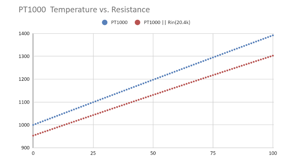
The image below shows the PT1000 curve with and without input resistor.

../../../_images/PT1000_resistance_1.png

In the curves below the polynomial coefficients are given as calculated in EXCEL.

SOMANET Node has an input resistance of 20.4 kΩ (for the single-ended analog input). This resistance is in parallel with the temperature sensor (PT1000). So the curve has to be redrawn with parallel input resistance in order to calculate the polynomial function coefficients.

../../../_images/PT1000_resistance_2.png

The equation below is related to the PT1000 temperature curve vs. PT1000 resistance|| Input resistance .

Temperature = -244 + 0.238x + 1.49E-05x² + 3.72E-09x³

$\Rightarrow$ a ₀ = -244, a ₁ = 0.238, a ₂ = 1.49E-05

The image shows how to add the coefficient in Node.

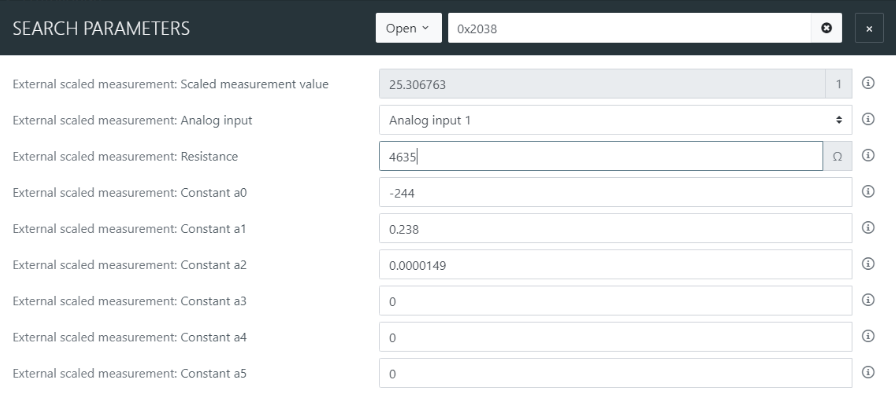
The accuracy of the measured temperature is related to the accuracy of all elements. For example, a 4.7kΩ resistor is set as the pull-up resistor but the measured value using a precise LCR meter is 4635 Ω.

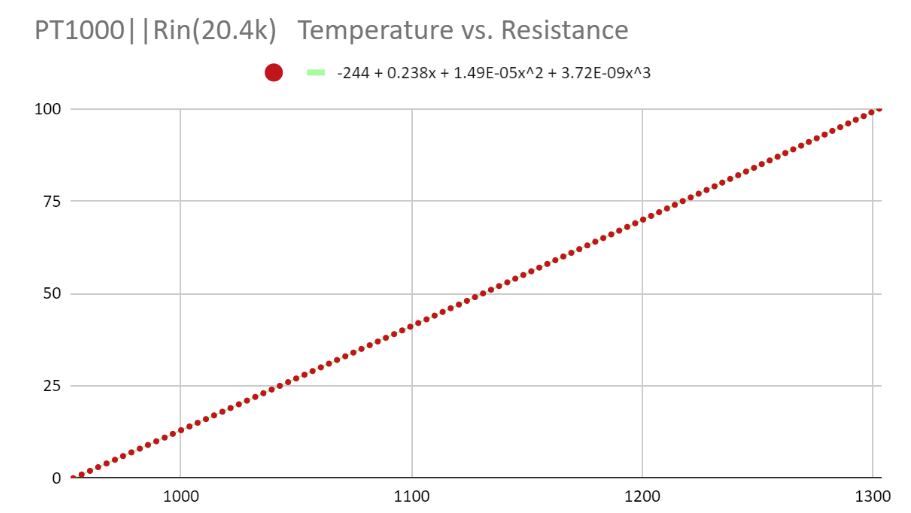
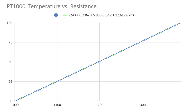
The image below shows the resistance vs. temperature curve for a PT1000 sensor.

Temperature = -243 + 0.236x + 5.93E-06x² + 1.16E-09x³

$\Rightarrow$ a ₀ = -243, a ₁ = 0.236, a ₂ = 5.93E-06

../../../_images/PT1000_resistance_3.png

If a higher sensitivity in a particular range of temperatures is required, the polynomial can be calculated only for that range of temperatures.

Note

For defining the protection level, one point is enough and the polynomial function is not required.

For example, the resistance value can be calculated for 90° in Node:

The resistance of a PT1000 is 1353 for 90° C, the input resistance of Node is 20.4 kΩ, and the resistance value and input value can be calculated:

$R_t = \frac {1353 \cdot 20400} {1353 + 20400}$ = 1268

For a polynomial function where a linear curve is considered, no complicated polynomial function is required.

The simple equation is $F(x) = a_1 \cdot x + a_0, a_1 = 1,a_2 = 0,a_3 = 0,a_4 = 0,a_5 = 0$

Defining the parameters a ₀… a ₅ will improve the accuracy by adding the sensor non-linearity in the temperature calculation.

Polynomial coefficients¶

It would be best if you use a temperature, pressure, torque… Vs. Resistance tables for extracting the polynomial coefficients.

In this example, we are going to extract the polynomial coefficient.

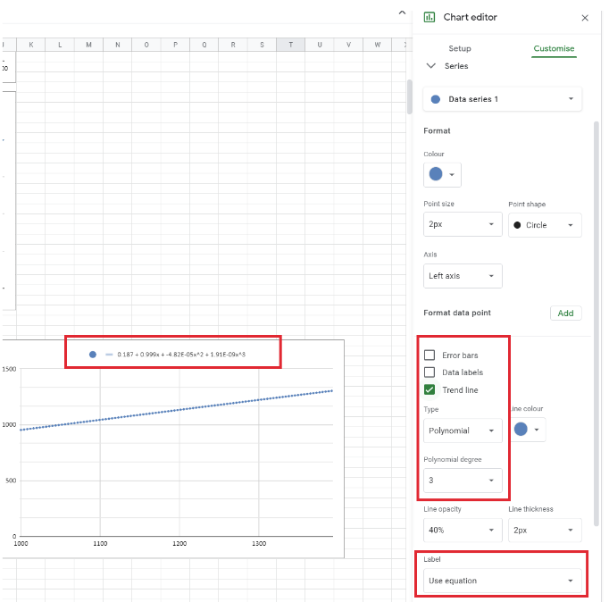
Follow the steps below for extracting the polynomial coefficient in Google spreadsheets:

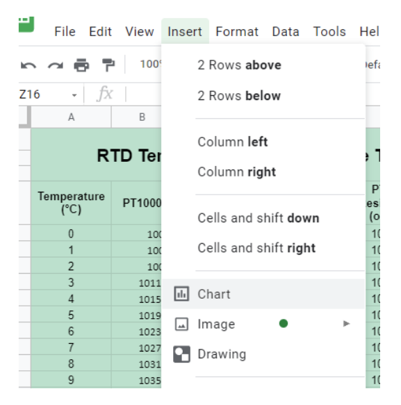
1 - Create the table.

2 - Insert the chart.

3 - Select the Scatter chart type in the chart editor menu in Setup.

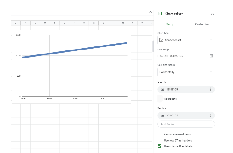
4 - In the chart editor menu select the series then select Trend lines.

5 - Then you can define the type of the line (polynomial) and polynomial degree.

6 - Use the equation as the label, then the polynomial function will appear on top of it.